Module datasheets often include current-voltage and power-voltage curves that show how the output power of the module decreases with decreasing irradiance. An example is shown in Figure 1, where we can see the peak of the power-voltage curves (thin lines) drop as the irradiance on the modules goes down from 1000 W/m2 to 600 W/m2. When the irradiance on the module is very low — as is the case when the module is fully-shaded — its power output is generally negligible. If this module is part of a string of panels connected to an inverter, it can cause the power of the entire string to drop. This is because the current through the string can only be as high as the current through the most shaded module, and as we can see from Figure 1, the current of a module (thick lines) decreases under shading.
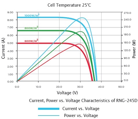
Figure 1: Current-voltage (thick lines) and power-voltage (thin lines) curves for a solar panel with varying irradiance. Image source: Savana Solar
This is the reason why manufacturers integrate bypass diodes into their modules. As an example, consider the case where nine out of ten modules are capable of outputting 8 A of current at a voltage of 32.5 V, but one of the ten modules is shaded and can only produce 1 A at about the same voltage. If the weak module is not bypassed, then the total output power is roughly 10 ⨉ 32.5 V ⨉ 1 A = 325 W, because the entire string is forced to operate at the lowest current (note that this assumes the unshaded modules still operate at 32.5 V; in reality it will operate closer to its open circuit voltage). If, however, we can bypass the shaded module, then the total output power becomes 9 ⨉ 32.5 V ⨉ 8 A = 2,340 W, excluding the small power loss due to the diode voltage drop.
But what happens if only part of the module is shaded? Does the whole module have to be bypassed, or can we use the unshaded sections to generate energy? It turns out you can, and this is why manufacturers integrate more than one diode into a module, effectively dividing the module up into smaller sections, called cell strings, each with a parallel bypass diode. When there is shade on only one of these cell strings, it can be bypassed while the rest of the module operates at maximum power. For a module with three cell strings (and three bypass diodes), that means we only lose about ⅓ of the module’s power instead of the entire module’s power when only one cell string of the module receives shade.
This is why it is important to analyze where there is shade on a module down to the cell string-level. Modeling solar designs to this level of granularity can have an appreciable impact on energy production results, and therefore expected financial returns.
How Submodule Simulation Affects Projected Returns on Commercial Projects
Consider the commercial rooftop in Figure 2, located in California (latitude 37.47°). We will design systems with varying row spacing, at 20° tilt to see how much DC power can fit in the limited area of the roof. The total system size for different row spacings are shown in Table 1, as are the module-level and submodule-level simulation results. As the row spacing is reduced, we can fit more modules on the roof, leading to higher energy production; however, as the rows get closer they begin to cast shade on each other (Figure 3). This means that while the overall energy production is increasing, the system efficiency, or energy yield (kWh/kWp), is reducing.
When simulating system performance at the module-level, Aurora bypasses a module if any point on the module is shaded. However, this does not necessarily reflect what would happen in the real world, where if only one cell string in a module is shaded — such as those along the bottom of a row of modules when in the shadow of the next row — only that cell string needs to be bypassed. Modeling at the submodule-level becomes increasingly important as the row spacing is reduced because it captures this behavior exactly.
The lack of granularity in the module-level simulation leads to an overly pessimistic NPV.
As the results in Table 1 show, the differences can be on the order of a few percent. This may not seem significant, but for a commercial solar project a small change in energy production can translate to a significant dollar value. The net present value (NPV) of each system, given the energy production results of module-level and submodule-level simulation, is shown in Table 2. The 2% difference in the performance estimate for the design with 1.5 foot row spacing leads to a 5.4% change in the NPV of the system, assuming a cost of $4/watt, a utility rate escalation of 3%, NEM (TOU) rates, an energy offset of ~80%, and a project life of 25 years. Also worth noting is that the NPV of the project increases as we reduce the row spacing, until we run a module-level simulation with the tightest spacing. The lack of granularity in the module-level simulation leads to an overly pessimistic NPV. This is not observed for the submodule-level simulation, where the energy production results for the tightest row spacing are more realistic.
Modeling at the submodule-level becomes increasingly important as the row spacing is reduced because it captures this behavior exactly. As the results in Table 1 show, the differences can be on the order of a few percent.
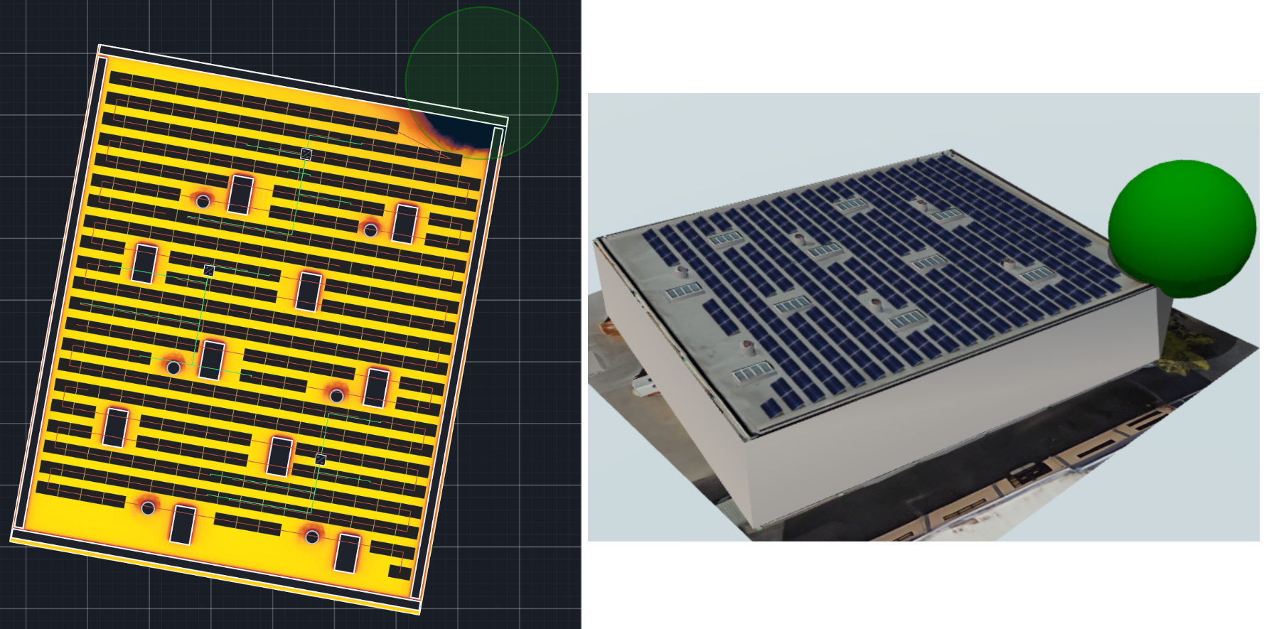 Figure 2: Small commercial site with an example system design and irradiance map showing shade from obstructions and parapet walls.
Table 1: System size and annual energy production results at the module-level (ML) and submodule-level (SL) for designs with decreasing row spacing.
| Row Sp. [ft] | DC Size [kW] | ML Prod. [MWh] | ML Yield [kWh/kWp] | SL Prod. [MWh] | SL Yield [kWh/kWp] | Diff. [%] |
|---|---|---|---|---|---|---|
| 3 | 65.52 | 103.21 | 1575 | 104.26 | 1591 | 1.01 |
| 2.5 | 70.20 | 110.30 | 1571 | 111.51 | 1588 | 1.09 |
| 2 | 79.56 | 123.43 | 1551 | 125.20 | 1574 | 1.42 |
| 1.5 | 84.24 | 127.08 | 1509 | 129.75 | 1540 | 2.08 |
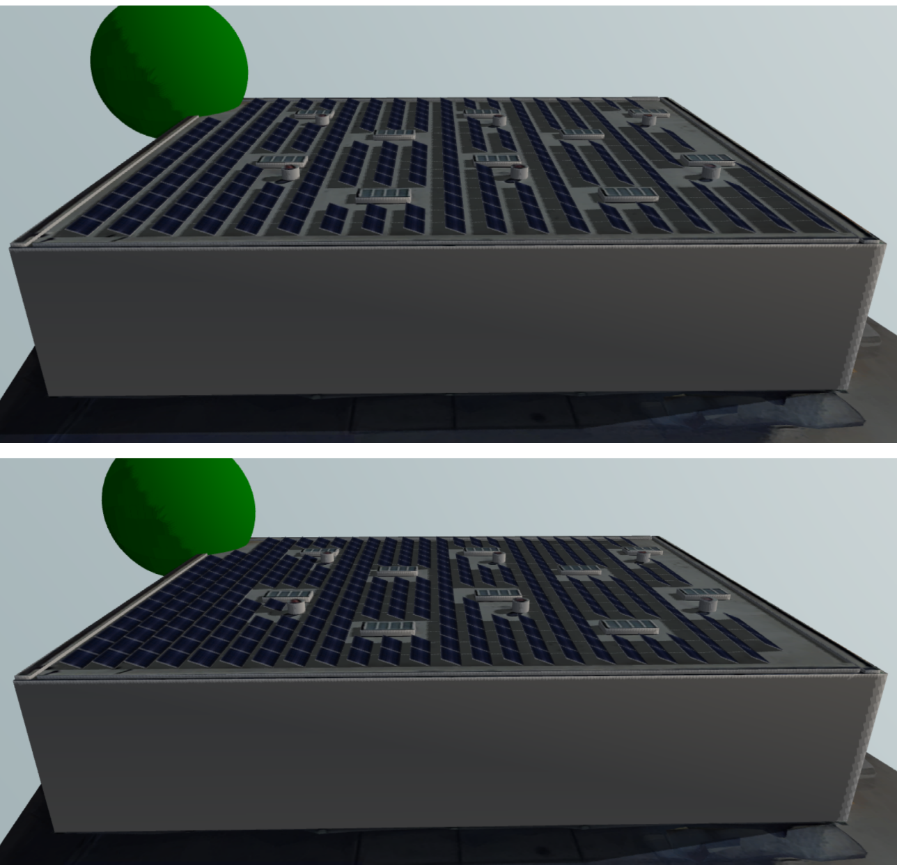 Figure 3: Aerial views of designs featuring 3 foot (top) and 1.5 foot (bottom) row spacing at noon in mid-December. Adjacent rows do not cast shade on each other in the design with larger row spacing, while there is significant inter-row shading in the design with narrower row spacing.
Table 2: Row spacing and net present value (NPV) at the module-level (ML) and submodule-level (SL) for designs with decreasing row spacing.
| Row Sp. [ft] | NPV, ML Simulation [$] | NPV, SL Simulation [$] | Diff. [%] |
|---|---|---|---|
| 3 | 62,689 | 64,092 | 2.21 |
| 2.5 | 66,388 | 67,933 | 2.30 |
| 2 | 72,933 | 74,769 | 2.49 |
| 1.5 | 72,209 | 76,218 | 5.40 |
Impacts of Submodule Simulation on Residential Designs
Accurately simulating a system at the submodule-level is important for the residential installer as well. Consider the design in Figure 4, which includes eight 255 W modules in series connected to a 3 kW string inverter. A module-level simulation gives an annual yield of 2.35 MWh, while a submodule-level simulation gives a result of 2.41 MWh — a difference of roughly 2.5%.
A module-level simulation gives an annual yield of 2.35 MWh, while a submodule-level simulation gives a result of 2.41 MWh — a difference of roughly 2.5%.
Of course, this is not a complete design for a house of this size. But it does serve to illustrate the importance of modeling at the submodule-level, especially under shaded conditions.
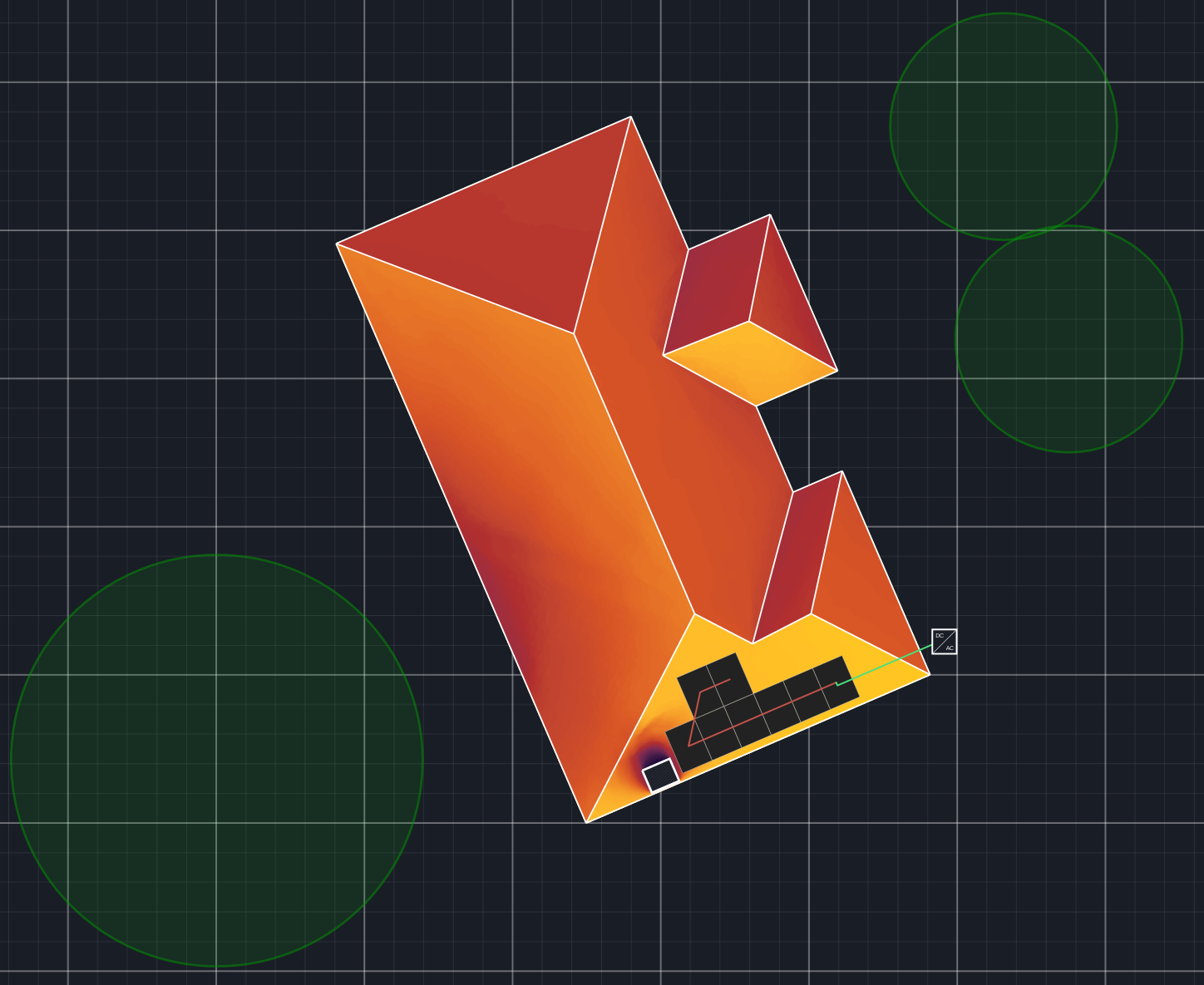 Figure 4: Design that includes a string of modules, with some modules experiencing concentrated shade from a chimney.
If the submodule simulation option is selected, Aurora’s performance simulation runs at the cell string level. The simulation algorithm takes into account exactly where on the module the shade falls and how the inverter bypasses shaded cell strings to maximize array power. Aurora makes no assumptions regarding the placement of bypass diodes inside the modules: we have contacted leading module manufacturers and confirmed exactly how they have configured their cell strings and bypass diodes, so our users can be confident that the simulation results accurately represent the systems they design.
To enable submodule simulation in Aurora, follow these instructions.
Takeaways:
- Bypass diodes inside modules are used to “skip over” shaded cell strings without bringing down the power output of the entire module (and string).
- Modeling the design down to the cell string level is necessary to accurately simulate the effects of bypass diodes, especially for commercial designs with inter-row shading.
- Submodule-level simulation can show production results 2% or greater (and closer to reality) than module-level simulation results.
- To enable submodule-level simulation in Aurora follow these instructions.
Want to see submodule simulation in action? Watch our webinar with Greentech Media: Improving Solar Energy Production Estimates with Submodule Simulation.